Optimizing Gradient Descent

15 Apr, 2025

Broadly speaking, gradient descent is the foundational algorithm for training neural networks. A lot of effort has gone into optimizing gradient descent (optimizing the optimizer) and in this blog post I want to:

Summarize the goal of optimizing gradient descent.
Look at a few popular optimizers and the concepts that underly them.
Touch on learning rate schedules.

Introduction

In modern day training of deep neural networks, mini batch stochastic gradient descent (MB-SGD) is the preferred optimizer. MB-SGD represents a compromise between SGD (efficient but noisy gradients) and GD (very inefficient but accurate gradients).

As great as MB-SGD is, it can still run into several problems during optimization:

The optimizer may get stuck in a poor local minima (DNN losses are non convex).
The optimizer may take too long to converge to a solution.
The optimizer may oscillate or diverge.

These problems not only impact the quality of the model being trained but also impact the amount of time it takes to train the model. In practice a lot of experimentation may be required before having a successful training run. Additional training time not only slows down engineering and research progress but it also results in higher training costs and higher energy consumption.

To address these problems researchers have come up with a variety of approaches (tricks) that have been shown to empirically outperform vanilla MB-SGD for certain problems. It’s also important to note that there is no single approach that is optimal for all problems (no free lunch).

Momentum and Adaptive Learning Rates

Two of the most important tricks in optimizing SGD (I will drop the mini batch prefix for brevity) are the ideas of momentum and adaptive learning rates, which we will expand upon here.

Momentum

The main idea behind momentum is best understood through a physics example (unsurprisingly). If we consider a ball rolling down a hill which then enters a flat spot, we will notice that momentum will keep the ball rolling along the flat spot. If the flat spot is not too long then the ball will pass through it and potentially enter another down hill.

The same idea when applied to SGD can help the optimizer avoid certain local minimas which can allow the optimizer to find better minima. Another way to think about momentum is that it allows the optimizer to take larger steps when going in a consistent direction which can help with converging faster.

Let’s take a look at the equations for SGD with momentum:

$$ \begin{align} m_t = \beta m_{t-1} - \eta g_t \\ \theta_t = \theta_{t-1} + m_t \\ \end{align} $$

The variable $m_t$ represents an exponentially decaying sum of past gradients from which we subtract the current gradient $g_t$ multiplied by the learning rate $\eta$. The hyperparameter $\beta$ represents the momentum and can have a value between 0 and 1. The closer $\beta$ is to 1 the more we emphasize the history of the gradient in our update and thus the more momentum we have. The closer $\beta$ is to 0 the less we emphasize our past gradients and thus the less momentum we have. A popular choice for $\beta$ is $0.9$.

Integrating momentum into our standard gradient descent update equation produces:

$$ \theta_t = \theta_{t-1} + \beta m_{t-1} - \eta g_t $$

In other words before we take a step in the direction of the negative gradient we first let our historical momentum move us in some direction.

Finally, I want to touch on why momentum can help speed up gradient descent in the case that the optimizer is consistently moving in roughly the same direction. This property falls out of the math of the exponentially decaying sum. If you assume that $g_t$ is some constant gradient and you compute a sequence of momentum vectors $\{m_t,m_{t+1},\cdots\}$ you will end up with a geometric series. Specifically the geometric series will have $a=1$ and $r=\beta$ which converges to $\frac{a}{1-r}$ or $\frac{1}{1-\beta}$. This means for $\beta=0.9$ we can end up with a momentum step that is 10 times as large as the gradient! That helps paint the picture of why momentum is so powerful and can help us step over local minima and cover a lot more distance per time.

Nesterov Momentum

One improvement to the above momentum formulation comes from Yurii Nesterov. Nesterov momentum makes one small change to the momentum we introduced above. Recall, in momentum we compute the negative gradient of where we are but prior to taking a step we first follow the momentum vector. Well with Nesterov momentum we compute the negative gradient after following the momentum vector. Nesterov momentum can speed up convergence.

Adaptive Learning Rates

Another idea for optimizing gradient descent revolves around adapting the learning rate based on the gradient. The motivation for this comes from the problem of doing gradient descent on a loss landscape that is elongated (flattish) in some direction. In that scenario normal gradient descent would follow the gradient down hill until reaching a relatively flat area which would then take many steps to traverse and reach a minima.

AdaGrad and RMSProp are two approaches that have been proposed for how to adapt the learning rate. For brevity we will look at RMSProp which is the better of the two. The basic concept of RMSProp is that when a gradient is very large we want to scale down how big of a step we take and when a gradient is very small we want to scale up how big of a step we take. If we followed this idea on an elongated bowl we would converge faster.

The equations for RMSProp are as follows:

$$ \begin{align} s_t = \rho s_{t-1} + (1-\rho)g_t^2 \\ \theta_t = \theta_{t-1} - \eta \frac{g_t}{\sqrt{s_t + \epsilon}}\\ \end{align} $$

Here $s_t$ represents an exponential decaying average of the square of the gradients with hyperparameter $\rho$ influencing how much older terms decay as well as the influence of the current gradient. The other hyperparameter $\epsilon$ is used to avoid division by 0.

In the gradient update step we see that it looks identical to regular gradient descent but with a term that we divide by. This term is effectively reducing the learning rate by a larger amount when the gradient is large and by a smaller amount when the gradient is small. If the gradient is really small the term could be less than 1 in which case it would actually increase the learning rate. This is consistent with the motivation for adapting learning rates!

Adam

The last type of optimizer we will cover is Adam (short for adaptive moment estimation) which essentially combines momentum with adaptive learning rates (RMSProp). While I haven’t checked whether Adam is still state of the art it seems like the common choice of optimizer in many publications.

Below is the algorithm as written in the original paper. Since we have already discussed the key components that Adam combines, it should be relatively easy to understand this algorithm.

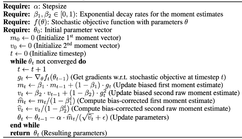
Let’s quickly review:

We can see the terms $m_t$ and $v_t$ correspond to the momentum and RMSProp terms we’ve already seen. Here they are referred to as the first and second (raw) moments, since they are a form of mean and (un-centered) variance.
Note $m_t$ slightly differs from our original momentum expression in that it is an expoentially decaying average (instead of just sum). The learning rate also ends up being multiplied by $m_t$.
Note we have parameters $\beta_1$ and $\beta_2$ which correspond to the momentum and decay hyperparameters.
Since our moments are initialized to 0, when we initially make updates to them the updates will be biased towards 0. The algorithm proposes correcting both moments by dividing by a term that eventually goes to 1 as $t$ gets larger. This effectively means that after a while there is no reason to perform the correction.

Finally, I wanted to note that there is an extension to Adam known as AdamW which shows that L2 regularization is not effective when used with Adam. AdamW proposes an alternative algorithm which has also been commonly adopted.

Optimizer Memory

One point that may not be immediately obvious about all of the optimizers we discussed is that they are applied per parameter. Since these optimizers depend on exponentially decaying averages of gradients and/or square gradients, each parameter will need additional memory to store its associated averages. This additional memory can add up for large networks!

Learning Rate Schedules

Prior to reading about learning rate schedules, I wondered why they are needed if optimizers like RMSProp and Adam effectively scale the learning rate. One insight is that the optimizers discussed are local – they only care about the gradients associated with a specific parameter.

Learning rate schedules, on the other hand, provide a way to set and adjust the learning rate globally for all parameters. The benefit of learning rate schedules is that they can (potentially) converge to a solution significantly faster than a fixed learning rate.

The challenge with a learning rate schedule is that we don’t want it to decay too quickly as that could result in a longer convergence time, but we also don’t want it to decay too slowly as that could prevent it from settling in a good minima. In other words we want to follow the Goldilocks principle.

Before looking at some of the most popular learning rate schedules it’s worth noting that learning rate schedules typically adjust the learning rate as a function of either the number of training epochs passed or the number of training iterations passed (e.g per mini-batch).

Some of the most popular learning rate schedules are:

Step, where the learning rate is decreased by some factor every $N$ iterations or epochs.
Exponential, where the learning rate is decayed exponentially over iterations or epochs (smooth).
Reduce on Plateau, where the learning rate is reduced by some factor when a metric (like validation loss) plateaus (stops progressing).
1 Cycle, where the learning rate ramps up to some maxiumum learning rate and then decays at a slower rate to some minimum learning rate.
SGDR, which uses cosine annealing to decay the learning rate but also has warm restarts where the learning rate jumps up to the maximum learning rate every $N$ iterations or epochs.

As with optimizers there will not be one learning rate schedule that is optimal for all problems, so experimentation is still key.

Conclusion

In this blog post we motivated the need for optimizing gradient descent which boils down to wanting to find the best solution in the least amount of time. We looked at the ideas of momentum and adaptive learning rates which feed into popular optimizers of the day like Adam. Finally, we (briefly) looked at a few learning rate schedules which have the potential to further speed up our training time.

A few closing thoughts:

The benefit of saving training time should not be underestimated since it can have a compounding effect.
Relatedly, it’s easy to imagine that for very large models these time savings could be measured in days if not weeks etc. As mentioned this really does save money and energy.
It feels like there is an ever growing list of design decisions we must make as deep learning practitioners. We now add two more decisions (optimizer and learning rate schedule) to the pile. The pile is too large to exhaustively try out all possibilities so instead we need some guiding principle. A few reasonable approaches may be:
- Start with the choices made by other researchers if your problem is similar in nature.
- Start with the simplest choices so as to establish a benchmark and then try advanced alternatives (e.g start with vanilla SGD and a constant learning rate).
- As budget allows compare different choices (e.g vanilla SGD vs Adam, constant learning rate vs step).
Deep Learning is really an experimental science, so experimentation is key!

References

Stat 453 Lecture by Sebastian Raschka – as usual lots of great educational material from Sebastian.