Reviewing Decision Trees

24 Mar, 2025

Decision Trees (and their ensemble counterparts) form another class of fundamental ML models and in this blog post I’d like to briefly review some of the key concepts behind them.

Introduction

The simplest way to think of a decision tree is that it is a tree which applies rules to an input and subsequently generates predictions that can be applied to both regression and classification problems.

When we make a prediction with a single decision tree on a test sample $\vec{x}$, we start by answering a sequence of questions about individual feature values of $\vec{x}$. These questions can be:

Is the numeric feature $x_i$ >= $3.2$?
Is the categorical feature $x_j$ == Sunny?
Is the ordinal feature $x_k$ < 3 Stars?

As each question in the tree is answered we traverse down the tree until reaching a leaf node. We can think of the leaf node as corresponding to the subset of training data whose features also have the same answers to these questions.

In other words, we have placed our test sample into the same bucket as a bunch of training samples and we then make a prediction about our test sample by aggregating the labels of the training samples in this bucket (gives off some K-NN vibes). If we are performing classification we may use majority voting for aggregation and if we are performing regression we may use averaging for aggregation.

Concrete Example

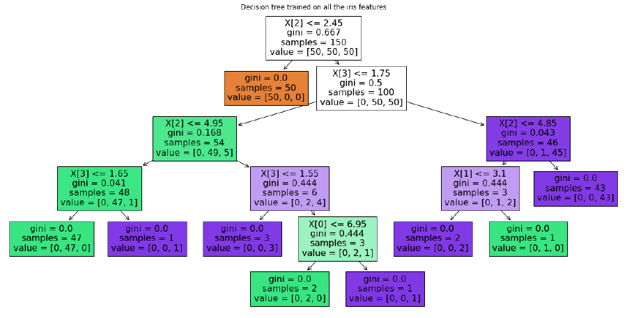
Let’s take a look at a concrete example where a decision tree has been trained for the problem of classifying iris plants. The training set consists of 150 samples each having 4 features (sepal length, sepal width, petal length, petal width) and a classification indicating which of 3 plant types the plant is (Setosa, Versicolour, Virginica). The decision tree that was learned for this problem is shown below (more on how it is generated later).

We see that the root of the tree asks whether the petal length is less than or equal to $2.45$. If our test sample answers this question as yes (True) then we proceed to the left child otherwise to the right child (False). In this tree the left child is a leaf node and if you land there then using the majority vote scheme you would predict the class as being class 0 (Setosa). If we land in the right child then we have another question to answer which is whether the petal width is less than or equal to $1.75$. Based on the answer to that question we would proceed down the tree until landing on a leaf node where we would make our prediction.

Example Decision Tree — Decision Tree for Classifying Iris Plants. (From scikit-learn docs.)

Training

At this point we have seen how you can use a decision tree to make a prediction. This leads to the obvious follow up question:

How is a decision tree constructed (or learned) and what is it optimizing?

Conceptually, we want a decision tree to ask questions that split the training data in such a way that leaf nodes are relatively “pure”. We can think of purity in the classification context as meaning a leaf node contains training samples that are predominantly of the same class (the closer to one class the more pure). In the regression context, purity would mean a leaf node contains training samples whose labels (target values) are similar to each other (the more similar the more pure).

Why do we want purity? Intuitively, if a decision tree has relatively pure leaf nodes, then we can argue the tree has learned patterns in feature space that are effective at discriminating between different classes or target values. Alternatively, consider a leaf node that is very impure, this would mean it contain samples that have very different semantics in which case we would argue the model hasn’t learned how to discriminate effectively and thus will not be useful for prediction.

Measuring Split Purity

When we actually train a decision tree, we will be evaluating splits (the questions posed by the tree). A split will be considered good if it produces children nodes that are relatively pure (compared to the parent). This brings us to the question:

How do we measure the purity of some node?

Classification

For classification, Gini impurity and Entropy are two of the most common measures of purity.

The Gini impurity score (opposite of purity) is given by:

$$ \begin{align} Gini(node) = 1 - \sum_{i=1}^k p_i^2 \\ \end{align} $$

Here $k$ denotes the number of different classes spanned by the samples in the node, and $p_i$ is the proportion of samples that belong to class $i$. We can see that if all samples are of the same class then the proportion for that class becomes 1 while all others become 0 leading to an impurity score of 0 (equivalently the most pure). Alternatively, if we had say $2$ classes and the samples were evenly split we would have an impurity score $0.5$ meaning not that pure.

Entropy, which will look familiar if you’ve also been looking at cross-entropy, is given by:

$$ \begin{align} Entropy(node) = - \sum_{i=1}^k p_i \log(p_i) \\ \end{align} $$

Here once again $k$ denotes the number of different classes spanned by the samples in the node, and $p_i$ is the proportion of samples that belong to class $i$. We can see that if all samples are of the same class then the proportion for that class becomes 1 while all others become 0 leading to an entropy of 0 (the most pure). Alternatively, if we had say $2$ classes and the samples were evenly split we would have an entropy of $-\frac{1}{2} \log(\frac{1}{2}) - \frac{1}{2} \log(\frac{1}{2}) = 1 $, indicating not pure.

Regression

For regression, a common way to measure purity is to use mean squared error (MSE). In this case we assume that a node will make a prediction ($\hat{y}$) that is equal to the mean target value of the $n$ samples in the node. The MSE of a given node is given by:

$$ \begin{align} MSE(node) = \frac{1}{n} \sum_{i=1}^n (\hat{y}-y_i)^2 \\ \end{align} $$

We can see when all samples in a node contain the same target value then the MSE will be 0. As the samples deviate farther and farther from each other (and thus the mean) the MSE will go up. Note in this case MSE is equivalent to the variance of the target values.

Optimization

So far we have characterized an optimal decision tree as one having relatively pure leaf nodes. It turns out that finding the most optimal tree (one that leads to the purest leaf nodes) is an NP-hard problem. It would require us to try all permutations of feature splits where the feature splits themselves depend on both the number of features and the range of values they can take on.

In practice decision trees are grown (trained) using greedy algorithms. The general flow of these greedy algorithms is as follows:

Initialize the root node of a tree by selecting the single split that provides the largest increase in purity (equivalently largest decrease in impurity) between root and the resulting children.
- The joint purity of the children can be evaluated by summing their individual purities weighted by the proportion of samples that belong to each child.
Next select a new split for each child that provides the largest increase in purity (or decrease in impurity) between it and it’s children.
Repeat the previous step (2) recursively until some stopping criteria is met or no further split can be found to increase purity.

The time complexity of the greedy algorithm is roughly $O(mn\log(n))$ where $n$ is the number of training samples and $m$ is the number of features. Some nuances on this time complexity are discussed here.

In practice there are a wide variety of decision tree training algorithms and some of the most popular ones are ID3, C4.5, and CART (comparison of them here). In general these different algorithms can vary in what kind of splitting measure they use, whether the splits are binary or n-ary, and how they perform pruning (see next section).

Regularization

One challenge with decision trees is that if you allow them to keep growing in size they can easily overfit to the training data. Therefore we look to several common regularization techniques that help reduce the freedom and complexity of the decision tree. These include:

Limiting the maximum depth of the tree. (Very common.)
Limiting the number of features being evaluated for each split.
Limiting the number of leaf nodes.
Setting a minimum number of samples for splitting to be allowed.
Setting a minimum number of samples a node must have in order to be created.

We can also think of these limits as forms of pre-pruning (proactively preventing the growth of the tree). There are also post-pruning techniques where you allow the tree to first grow without restriction and then afterwards nodes are pruned.

Pros and Cons

There are several pros and cons to consider before applying decision trees to your problem.

Pros:

One of the biggest pros is that decision trees are interpretable. For any particular leaf node you can find the path from the root to it and this path represents a sequence of interpretable questions and answers (rules) that led to a certain prediction. Interpretability is really important in many domains including healthcare, criminal justice, and autonomous systems.
Decision trees can provide insight into feature importance. That is we can look at how much purity was gained when splitting on a particular feature and use this as a signal of which features are most important. This again gets back to the idea that features that can help discriminate between classes/labels are more important than those that do not.
Decision trees can happily work with mixed data types.
You don’t need to worry about scaling/normalizing input features.
Decision trees are relatively robust to missing feature values (e.g when growing a tree samples with a missing feature value can be ignored).

Cons:

Decision trees by nature make splits that are orthogonal to the axes (e.g $x < 3$ or $y > 5$) which means that the results of a decision tree can be sensitive to the orientation of the data. If some decision boundary is not axis aligned (e.g a diagonal one) then it will be harder to model it cleanly and will generally require a larger decision tree. Rotating your data with PCA may help with this problem but there is no guarantee.
Decision trees are very prone to overfitting. This means small changes to the training data (or hyperparameters) can lead to very different models. We will see that ensemble models can help to reduce the variance of the model.

Ensemble Learning

In ML there is a powerful concept where you can often come up with a better performing model by aggregating the predictions from multiple different models. This general concept is known as ensemble learning and can be informally thought of as “the wisdom of the crowd” (not necessarily the most intuitive).

In this section I will give an extremely brief overview of a few popular approaches for ensembling decision trees.

Random Forests (Bagging)

Some of the most successful applications of decision trees have been in the form of ensembles. Ensembles of decision trees can lead to better performance and reduce model variance. One of the most popular methods of ensembling decision trees is called random forests.

In general, random forests use two strategies for creating an ensemble of different decision trees:

The first is that each decision tree is trained using a different subset of training data. The subset of training data is usually generated by sampling with replacement and leads to a diversity of trees since they each model different datasets. This overall approach is known as bagging (short for bootstrap aggregating).
Additionally, when growing the decision trees, each tree will only consider a random subset of features when determining the best splits. This further helps to decorrelate the different trees since they will make predictions based on different features.

One advantage of this kind of ensembling technique is that it lends itself well to parallelization. Each tree in the ensemble can be trained independently!

AdaBoost and Gradient Boosting

Another popular way to ensemble decision trees is to construct them sequentially so that later trees can learn to correct the mistakes of previous trees. This strategy is broadly known as boosting with two of the most popular methods being AdaBoost and gradient boosting (e.g XGBoost).

At a very high level AdaBoost creates an ensemble of trees by identifying which training samples were misclassified (or had a large error in the regression context) and increasing the weight of those samples so that they become more influential in the construction of the next tree (e.g the optimal split is influenced more by those samples).

Like AdaBoost, gradient boosting creates a sequence of decision trees but instead of changing the weights of training samples, the objective is instead to have subsequent trees fit the errors of their predecessors directly. Gradient boosting has shown to still be state of the art for many prediction tasks on tabular data.

Conclusion

In this blog post we’ve looked at the fundamentals of decision trees which are fairly distinct from other classic models like linear regression, logistic regression, and neural networks.

Decision trees have many advantages as we discussed, but need to be constrained to avoid overfitting. They are a popular choice for base model in ensembles which are often the go to model when working with tabular data. There is a lot more depth behind the various ensembles we touched on which cannot be covered in this post. For additional reading I’d recommend diving into gradient boosted trees.