Vision Meets Transformers
When I began my PhD in computer vision the leading approaches of the day were models like support vector machines, probabilistic graphical models, and decision trees. Fast-forward to 2016 when I was graduating and the deep learning revolution was underway. Leading approaches were convolutional neural networks like AlexNet, VGG, and ResNet.
I had the fortune to play with CNNs for the final project of my PhD. Specifically, I experimented with finetuning a VGG-16 CNN on a very small dataset for the task of pose estimation. The results weren’t very good which I think was due to a combination of having a very limited training set and targeting a domain too different from the source domain. I was working with grayscale images of moths captured in a laboratory which looked nothing like the ImageNet images used to train the base model.
Since graduating and entering industry my career moved away from computer vision and so I stopped attending (LLM pun intended) to where the field was headed.
In this blog post I briefly review a few papers that seem important for understanding the field of computer vision as it is today. A motivating question for finding these papers is asking how have transformers been used for vision problems?
Vision Transformer
In research it’s very common to look at successful approaches in one area and try them out in another. So it’s no surprise that following the success of transformers in NLP some Google researchers published a paper applying the transformer to the task of image classification. The paper showed that a transformer could outperform CNNs on image classification tasks while using less compute.
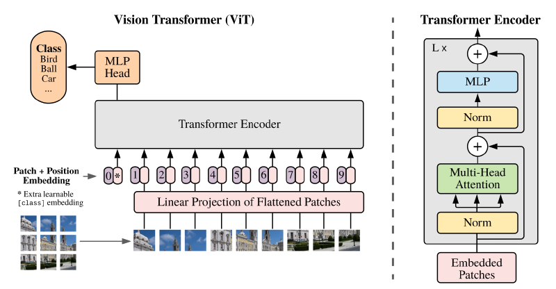
Zooming in a little, we see that in order to apply a transformer to an image we need some way to turn it into a sequence of vectors. The approach taken in this paper is to slice up an image into small patches (e.g \(16\times16\) pixels.), flatten each patch, and then order them from top to bottom and left to right. Then a learned linear projection is applied to each image patch to produce embeddings. Positional embeddings, which are learned, are added to the input (image) embeddings. The resulting vectors are fed into a transformer encoder.
In order to perform classification a classification head was added to the transformer encoder along with a classification token (learnable embedding) at position 0. During training, large labeled image datasets (like ImageNet and successors) were used with a standard classification loss to train the model (in contrast to pre-training with self-supervision). The authors report that when fine-tuning for specific tasks the pre-trained prediction head is replaced by a zero initialized feed forward layer. The overall architecture is shown in the figure below.
Another important point this paper made is that transformers didn’t do better than CNNs on smaller datasets like the original ImageNet (~1M images). It wasn’t until they used a ~300M image dataset that the transformer clearly outperformed CNNs. One reason why transformers may need to see a lot more data before they are competitive with CNNs is that they don’t have the same inductive bias. CNNs are designed to learn patterns (filters) that are translationally invariant. This is useful because objects can appear anywhere in an image and so you want a model to learn the general concept while largely ignoring where globally the pattern appears.
One cool thing to see from the paper is the visualization of the linear projection that is learned by the model. The visualization shows lower level edge and blob like patterns which look similar to what you would expect is learned in the earlier layers of a CNN. We can then think of this linear projection as extracting features from the images.
Detection Transformer (DETR)
Another early work in leveraging transformers for vision is the Detection Transformer (DETR) paper from Facebook. At a high level the paper demonstrates that you can leverage transformers to predict in parallel a set of bounding boxes (and classes) and do well at object detection while using a simpler architecture than some of the earlier state of the art approaches (like Faster R-CNN). They also demonstrate results for the problem of segmentation.
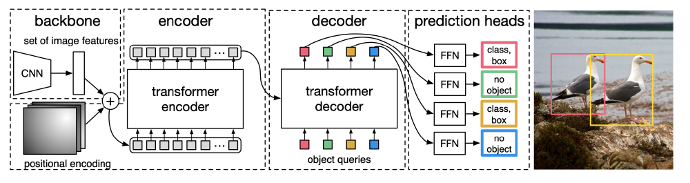
Once again, zooming in a bit we see that the paper brings together several ingredients including a CNN, an encoder-decoder transformer, and a feed forward network to predict individual bounding boxes and classes.
The CNN applies a large number of filters (e.g 2048) to the input image which results in a large number of lower resolution outputs/responses. These lower resolution activation maps are reduced from having \(C\) filters to \(d\) filters/dimensions. After reshaping these outputs we get a sequence of \(HW\) \(d\)-dimensional vectors, where \(H\) and \(W\) are the height and width of the outputs. We can then think of this sequence as as a sequence of image features corresponding to different parts of the image which are then fed into an encoder transformer.
The encoder output is then available for use by the decoder whose outputs are fed through a relatively shallow FFN to predict bounding boxes and classes. A really important aspect to training this model is that predicted detections need to be compared to ground truth objects. In order to do this comparison you want to first identify which pairs of predictions and ground truth objects go together. This is done using the hungarian algorithm which performs bipartite matching such that the matching cost is minimized/maximized. In order to allow the model to predict all of the objects in an image they choose a value \(N\) that represents the largest number of objects expected in an image. If the actual number of objects is below \(N\) then dummy “no object” objects are added to the ground truth object set so that surplus predictions can be matched in the bipartite matching. An illustration of the overall model is shown below.
One interesting quirk in this paper is deciding what inputs the decoder should receive. We know that the decoder can gain a good understanding of different parts of the image by attending to encoder outputs. We also know that decoder outputs should represent various object predictions. The authors chose to simply treat these decoder inputs as learnable positional embeddings (which they refer to as object queries). The main intuition for this seems to be rooted in the requirement that the input vectors need to be distinct from one another. We can see this is needed because if all inputs were identical then the result of both self attention and cross attention would be identical for every vector ultimately leading to the same exact object prediction from each decoder output. Given that distinct values are needed the authors decided the specific choice can be left to the model to learn. It makes sense that the model would learn distinct object queries because otherwise the loss function would heavily penalize repeated object predictions (as only one could possibly be matched to the right object).
Conclusion
These early works which apply transformers to computer vision demonstrate that with large quantities of data and compute you can get state of the art performance. In many ways this isn’t surprising given the enormous success of transformers in modeling language. Does this mean that transformers are better than CNNs for all real world vision applications? Of course not! You have to pick the right tool for the application and its constraints.
References
- Vision Transformer (ViT) Paper
- Detection Transformer (DETR) paper
- DETR YouTube Video - Nice video on the paper from Yannic Kilcher.