Bias and Variance
One way to view different ML models is through the lens of bias and variance. In this blog post I want to summarize the concepts of bias and variance and address several questions I had after writing about decision trees.
Concepts
At a high level bias and variance are two attributes of a model that influence the errors the model will make on unseen data.
We will start by definining bias and variance at a conceptual level and then we will look at some math that details how each contribute to the expected error a model will make on unseen data.
Bias
The bias of a model can be thought of in terms of how well the model’s assumptions match the underlying function that generated the data (which is unknown to us).
If for example we have data generated by a sinusoidal function like \(y=sin(x)\) and we fit the linear model \(\hat{y}=w_0x+w_1\) to it, we would say our model has a high bias as it makes assumptions that don’t match the underlying function that generated the data. High bias is synonymous with underfitting and we would expect such a model to make erroneous predictions.
If on the other hand we chose a model that was a sinusoid (with the right frequency), then we would say our model has low bias. Low bias would tell us we have a model that generally fits the data well.
Variance
Variance is a little bit trickier to think about it. We can think of variance as measuring how sensitive a model is to small changes in the training data. High variance is synonymous with a model that overfits to the training data. Overfitting means the model begins to fit to noise contained in the training set. We would expect a model with high variance to also make erroneous predictions on unseen data.
Mathematical Definitions and Decomposition
Now let’s look at the mathematical definitions of bias and variance for which we need to introduce a thought experiment:
- Suppose we have \(N\) different training sets each randomly sampling from a broader training set (e.g via bootstrapping).
- Suppose we then train a regression model on each of the \(N\) training sets, yielding \(N\) models.
- Suppose we then use each model to make a prediction for some data point \(x\), yielding predictions \(\{\hat{f_1}(x),\hat{f_2}(x),\cdots,\hat{f_{k}(x)}\}\).
- Now think of our model \(\hat{f}\) as a random variable that can make different predictions due to the underlying training data used to train it.
Now we are ready to define bias and variance mathematically.
Bias
Bias is defined as the difference between the expected model prediction and the ground truth value \(f(x)\). Notice that even if the predictions are all over the place, so long as their mean is close to \(f(x)\) the bias will be low.
$$ Bias(\hat{f}(x)) = \mathbb{E}\big[\hat{f}(x)\big] - f(x) \\ $$Variance
Variance is defined by looking at the square of how much the predictions deviate from the mean prediction, and then taking the mean across different predictions. The higher the variance the more wildly the predictions will vary from one training set to another.
$$ Var(\hat{f}(x)) = \mathbb{E}\big[ (\hat{f}(x)-\mathbb{E}[\hat{f}(x)])^2\big] $$Decomposition
The most common way that bias and variance are presented mathematically is by showing how they each contribute to the MSE (regression context), which represents the model’s expected prediction error. In other words the MSE considers all possible predictions we could make and tells us how big the squared error would be in expectation.
$$ MSE(x) = \mathbb{E}\big[ (f(x) - \hat{f}(x))^2 \big] \\ $$If we expand out the definition for MSE we get the following:
$$ \begin{align} = \mathbb{E}\big[ (f(x)^2 - 2\hat{f}(x)f(x) + \hat{f}(x)^2 \big] \\ = \mathbb{E}\big[ f(x)^2 \big] - 2\mathbb{E}\big[\hat{f}(x)f(x)\big] + \mathbb{E}\big[\hat{f}(x)^2 \big] \\ = f(x)^2 - 2f(x)\mathbb{E}\big[\hat{f}(x)\big] + \mathbb{E}\big[\hat{f}(x)^2 \big] \\ = f(x)^2 - 2f(x)\mathbb{E}\big[\hat{f}(x)\big] + \mathbb{E}\big[\hat{f}(x)^2 \big] - \mathbb{E}\big[\hat{f}(x)\big]^2 + \mathbb{E}\big[\hat{f}(x)\big]^2\\ = f(x)^2 - 2f(x)\mathbb{E}\big[\hat{f}(x)\big] + \mathbb{E}\big[\hat{f}(x)\big]^2 + \mathbb{E}\big[\hat{f}(x)^2 \big] - \mathbb{E}\big[\hat{f}(x)\big]^2 \\ = (\mathbb{E}\big[\hat{f}(x)\big] - f(x))^2 + \mathbb{E}\big[\hat{f}(x)^2 \big] - \mathbb{E}\big[\hat{f}(x)\big]^2 \\ = Bias\big(\hat{f}(x)\big)^2 + Var\big(\hat{f}(x)\big) \\ \end{align} $$This decomposition of the MSE is known as the bias variance decomposition. The reason it’s useful is that it shows us concretely how bias and variance influence the expected generalization error. We can see that bias has an outsized impact on the generalization error and variance also contributes. For simplicity the above derivation leaves out the irreducible noise component which represents the noise intrinsict in our training data which we can’t remove.
It’s also worth noting that for other kinds of errors/losses there are other bias variance decompositions (see here).
The Tradeoff
Bias and variance are often thought of in terms of trading off one for the other. For example if you have a high bias model you may reduce the bias by choosing a more flexible model which can better fit the training data. However, the more flexible model may be more prone to overfitting the data because of its flexibility and so we end up trading bias for a higher variance.
The opposite direction is also true, if we have a model that is overfitting with high variance we may choose a less flexible model and give up some bias in exchange for lower variance.
The figure below shows this tradeoff along with the decomposition of MSE.
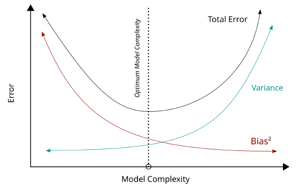
As practitioners our goal is to choose a model that has a good balance between bias and variance. In other words we need to avoid underfitting and overfitting!
Reducing Variance
In my previous blog post on decision trees, I mentioned that ensembles of decision trees can result in a model with reduced variance. This led me to wonder how exactly do ensembles reduce variance?
Well, it turns out my initial statement was a bit too broad. It’s more accurate to say that specific ensembling techniques like bagging and random forests were designed to reduce variance. On the other hand, ensembling techniques like boosting were designed to reduce bias. It’s also possible that an ensembling technique may reduce both bias and variance but it would depend in general.
With that clarification out of the way the revised question becomes:
How do ensemble techniques like bagging and random forests lead to models with lower variance than their constituents?
The main insight to answering this question comes from looking at what happens if we take a pair of random variables and compute the variance of their average?
Averaging Model Predictions
Suppose, we had two models whose predictions (random with respect to training dataset choice) are modeled as random variables \(X\) and \(Y\).
What would happen if we averaged the predictions of the two models and computed the variance of this average?
$$ \begin{align} Var\big(\frac{1}{2}X + \frac{1}{2}Y\big) \\ = \frac{1}{4}Var(X) + \frac{1}{4}Var(Y) + \frac{1}{2} \; Cov \; (X,Y) \end{align} $$The second line follows from the properties of variance (see wiki). Now let’s bring correlation \(\rho\) into the picture:
$$ \rho = \frac{Cov\;(X,Y)}{\sigma_x\;\sigma_y} $$If we re-arrange for covariance and substitute into the prior equation we get the following expression for the variance of the average:
$$ \begin{align} = \frac{1}{4}Var(X) + \frac{1}{4}Var(Y) + \frac{1}{2} \; \rho \; \sigma_x \; \sigma_y \\ = \frac{1}{4}\sigma_x^2 + \frac{1}{4}\sigma_y^2 + \frac{1}{2} \; \rho \; \sigma_x \; \sigma_y \end{align} $$If we assume the models have identical variance then we get:
$$ \begin{align} = \frac{1}{4}\sigma^2 + \frac{1}{4}\sigma^2 + \frac{1}{2} \; \rho \; \sigma \; \sigma \\ = \frac{1}{2}\sigma^2 + \frac{1}{2} \; \rho \; \sigma^2 \end{align} $$Now, we see that there are two terms that characterize the variance of the average prediction:
- The first term shows that the predictor obtained from averaging has half the variance of either individual predictor (assuming equal variance).
- The second term shows that when the predictors have 0 correlation then the total variance is just the first term. If there is some correlation (less than 1) then the variance increases proportionally but will still be reduced relative to each individual predictor.
Finally we have the mathematical intuition as to why averaging predictors can result in a predictor that has lower variance and this is the answer to our question.
Wrapping Up
We have shown why taking an average across multiple predictors can result in a predictor with lower variance. Now let’s connect it back to decision trees which motivated this blog post.
- Decision trees tend to have high variance due to their flexiblity to fit data. We would like to reduce variance so that our model can generalize better.
- Bagging decision trees implies training multiple trees on different bootstraps and making a prediction by averaging predictions from individual trees. We now understand why this reduces variance.
- However, trees in a bag are still likely to be fairly correlated which reduces how much the ensemble reduces variance.
- Random forests address this problem by further decorrelating the individual predictors (decision trees). This is achieved by randomly choosing which subset of features are available to split on at a particular node.
Conclusion
In this post we’ve looked at bias and variance from a conceptual and mathematical view. We’ve also shown mathematically why ensembling (in specific ways) has the potential to reduce model variance.
References