Oops, Contrastive Representation Learning

Originally I wanted to focus this blog post on a vision + transformer paper known as DINO. I quickly realized that I would need to recurse into background reading before I could understand DINO. So instead this post will be about contrastive representation learning and several other papers which will help with understanding DINO. Hence the title beginning with Oops.

We’ll begin by reviewing contrastive representation learning which will set the stage for a few important papers.

Contrastive Representation Learning

There is this broad concept that if we have a bunch of data points (e.g images) we would like to be able to learn a good representation of them. One way to set this up as a learning problem is to encourage similar data points to be closer together in the representation space and unlike data points to be farther appart.

One place where I had seen this broad concept was in the Locality-Sensitive Hashing (LSH) paper, which I encountered in grad school. The general idea is that you want to preserve relative distances of data points in their original space when coming up with a “good” low dimensional representation.

Another work I encountered in the past was FaceNet where they learn representations of faces by encouraging faces from the same person to be closer in representation space than faces from two different people. They introduce a triplet loss, illustrated below, which encodes this objective.

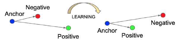
The triplet loss says that some person’s face (represented by an anchor) should be closer in representation to some other photo of their face (represented by the positive sample) than to some photo of someone elses face (represented by a negative sample). This is a triplet loss because the loss requires three representations (anchor, positive, negative) to be computed. You’ll also notice in the paper that there is a hyperparameter \(\alpha\) which is used to set a margin, meaning the distance between anchor and negative must be at least \(\alpha\) more than the distance between anchor and positive. The representation is also constrained to have a magnitude of \(1\).

We can think of this triplet loss as an example of supervised contrastive representation learning since the loss depends on the identity of a face image which is provided by labels. Next we look at the SimCLR paper which requires no labels and is an example of self-supervised contrastive representation learning.

A Simple Framework for Contrastive Learning (SimCLR)

SimCLR proposes a framework to apply contrastive learning to images without the need for labels and hence it is a self-supervised approach. In general I would expect self-supervision to outperform supervision because it enables using a lot more data and the signal for training is not limited to labels which could be relatively shallow (e.g describing a rich image with a single label).

In the image below we see the main idea behind self-supervised contrastive learning.

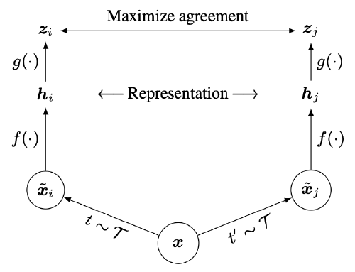
• First we take an image \(x\) and apply two different random transformations (image augmentations) to them (e.g cropping, blurring, color distortion).
• Then you feed the two different augmentations through some encoder \(f\) (often chosen to be ResNet) which produces a representation \(h\).
• You then feed the representation through a small neural network (\(g\)), referred to as a projection head, which produces a vector \(z\).
• A contrastive loss is then defined which takes as input the two final representations \(z_{i}\) and \(z_{j}\) (each representing a different augmentation of the source image).

The loss, similar to what we’ve seen before, encourages the representations of the augmentations for the same source image to be very similar to each other, while being dissimilar from the other augmentations in the batch. If we further zoom into the loss formulation in the paper we see the following:

• Looking at the paper the similarity between two representations is taken as the cosine distance which is the dot product of the normalized vectors.
• We also see the loss is of the form \(l_{i,j}=-log(num/den)\) which means we want the denominator to be small so that the fraction is larger and the \(log\) is larger and therefore the loss is smaller.
• The denominator is a sum of similiarities between \(z_{i}\) and all representations in the batch from other source images. This means the loss encourages \(z_{i}\) to be dissimilar to all augmentations from other source images in the batch. (Small aside the paper is confusing because it appears \(z_{j}\) is included in the denominator in the equations, despite the text saying that negative examples come from the other \(2(N-1)\) examples. Perhaps it doesn’t really matter whether it is included or not?).
• Finally we see that the total loss is the average of individual losses \(l_{i,j} + l_{j,i}\) for \(N\) source images in the batch. Notice that \(l_{i,j}\) alone is not symmetric due to the denominator but if you add \(l_{j,i}\) then you do have a symmetric loss.

After training the model, what you end up using is just the encoder \(f\), while the projection head is discarded. This encoder \(f\) should then be able to produce representations of images that are useful for downstream tasks. Indeed SimCLR demonstrated that their representation combined with a linear classifier outperformed other techniques on classifying ImageNet images.

Bootstrap Your Own Latent (BYOL)

Now we’re going to look at a paper that outperforms SimCLR but is similar in design and so our understanding of SimCLR will be very helpful here.

BYOL, like SimCLR, aims to learn a “good” image representation without the need for labels. We again define a representation to be “good” if it can be used to perform many downstream tasks well.

The way BYOL works is depicted in the figure below and it involves the following steps:

• Take an image \(x\) and perform two different data augmentations on it, leading to \(v\) and \(v'\).
• Input each augmented image into two different neural networks, one having parameters \(\theta\) which is part of the “online” network and the other \(\xi\) which is part of the “target” network. In the paper these neural networks are ResNet CNNs.
• The online network has two additional MLPs that follow the ResNet. The output of the online network can be thought of as some function of \(z_{\theta}\), where \(z_{\theta}\) is a lower dimensional representation of the first augmented image \(v\).
• The target network has one additional MLP that generates a lower dimensional representation of the second augmented image \(v'\) called \(z'_{\xi}\).
• Now the goal is for the two networks to output the same vector which is what the loss function is designed to encourage. There are also several interesting quirks about training:
  • Only the online network is trained. In other words each training step only modifies the weights \(\theta\).
  • The target network weights are taken as an exponential moving average. In other words the target network weights are updated to be a combination of itself and the latest online weights.
• Lastly, after training most of the architecture is thrown away. The only part that is kept is the now trained ResNet which hopefully has learned to produce a “good” image representation.

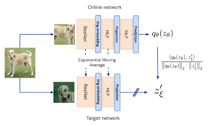
My high level understanding of this model is that like SimCLR it learns that different augmentations of an image don’t change the underlying meaning of the image. If we learn a good representation for the original dog image then we would expect the two augmentations to be related by a relatively simple function (represented by \(q_{\theta}\)).

One important difference between BYOL and SimCLR is that BYOL does not make use of any negative examples. This is not only an improvement in terms of computation but it also avoids having to worry about some of the nuances of how you pick the best negative examples to use. You also don’t need to use as large of a batch size which is more important in SimCLR where you do need good negative examples.

If we think about why negative examples are used in the first place it’s to help the learning process by not just saying what should be similar but by also saying what should be disimilar. You also prevent the model from just outputting the same vector for every single input since that would be violating the dissimilarity part of the loss.

This leads to the mystery of this paper which is how the model prevents the networks from learning a trivial solution (known as mode collapse) to the problem given that there are no negative examples being used. The authors state that in practice the model does not converge to the trivial solution and so in practice this problem does not arise.

What I also found a bit challenging to wrap my head around initially is that there are two networks with different parameters but one kind of tracks the other. However after reading SimCLR, which I originally read after BYOL, it isn’t as weird since SimCLR can be thought of as using the same network twice with the same parameters, this is more of a tweak on that.

For this paper I once again recommend the commentary from Yannic Kilcher’s YT Video which helped my understanding of the paper.

Conclusion

Writing this blog post was pretty helpful for me because I hadn’t been exposed to self-supervised representation learning in the vision domain.

Stay tuned for my post on DINO. My post on DINO is now up!

References

• SimCLR
• Bootstrap Your Own Latent (BYOL)
• BYOL YT Video Another helpful video from Yannic Kilcher’s YT page.